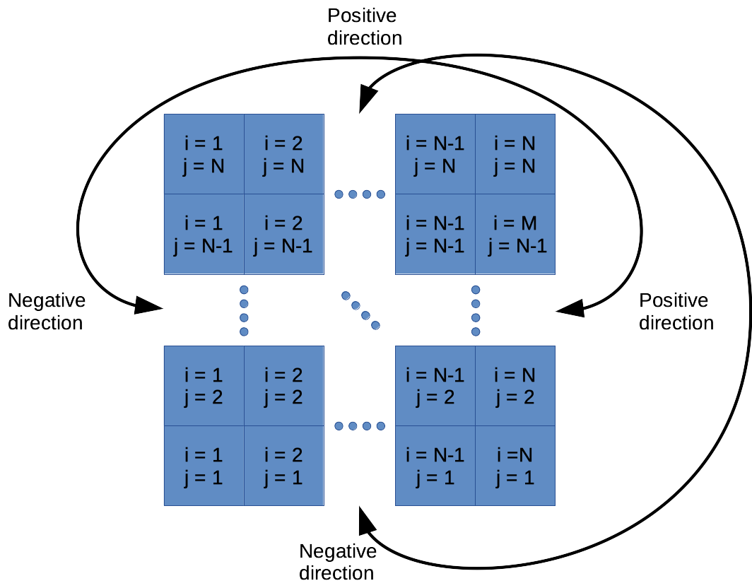
CyclicArrays

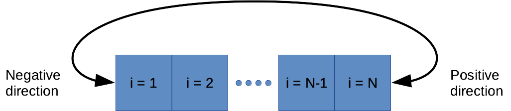
CyclicArrays allow for the intuitive definition of a circular domain composed of one or more arrays, where the faces of the arrays are interconnected. Each array will have two directions (positive and negative) and up to three space dimensions (x,y,z). After the definition of the connection between different faces, out-of-boundary indexes will be permitted. The CyclicArray structure includes two fields - data array and connection array. The data array containing the data values and the connection array containing the information on the connections between faces and their sides.

–- CyclicArrays.jl is a generalization of CircularArrays.jl package for various grid topologies (see section Connections below for more details) –-

Quick example

Start predefined 1D array:

using CyclicArrays
x=[0:3;]
x1=CyclicArray(x,"1D")

This will output:

4-element CyclicArray{Int64,1}:
   [0, 1, 2, 3]

Then:

x1[0:5]

Output:

6-element Array{Int64,1}:
 3
 0
 1
 2
 3
 0

The connection array

The connection array is a four-dimensional array defining the connections between faces:

Array dimension - 1:(number of arrays)
Spatial dimensions, size up to three - x=1, y=2, z=3
Direction, size 2 (negative direction = 1, positive direction = 2)
Target - four values that point each array, dimension, and direction to its neighbor. The first three values indicate the neighbor array, dimension and direction. The fourth value indicates whether there is a need to flip the face upside-down (0 - no-flip, 1 - flip).

Several predefined connection array are available with the method:

CyclicArray(x::AbstractArray,str::String)

Connections

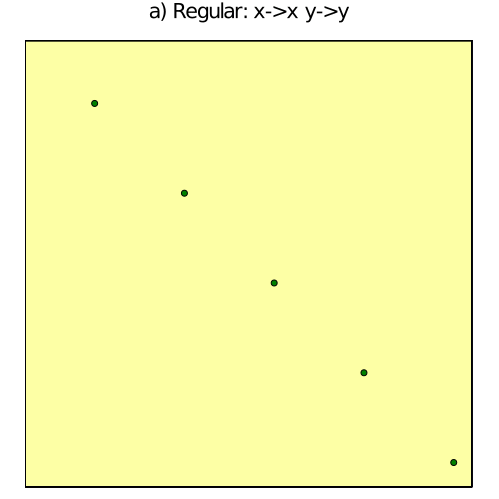
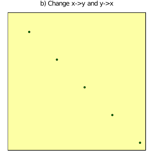
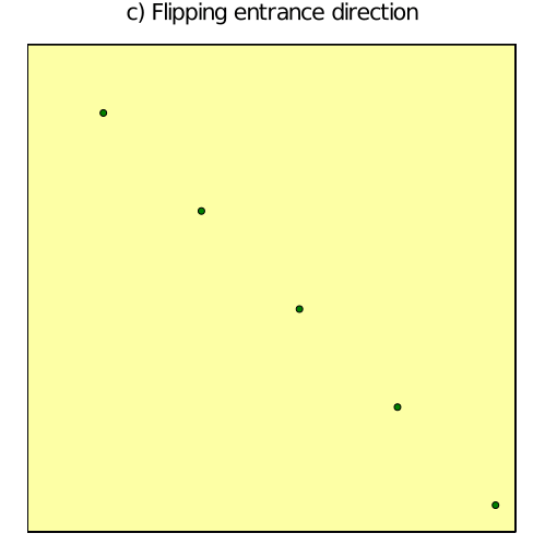
The generality of CyclicArrays allows for the generation of various grid types. Below are three examples, each with five moving particles.

The first example (a) shows the trivial case where a particle that exits the right edge enters from the left. Similarly, a particle that leaves the top edge enters from the bottom.
Animation (b) shows a case in which the x-y directions are switched. When a particle exists from the right edge (x-direction), it enters from the bottom edge (y-direction). When a particle exits from the top edge, it enters from the left.
Animation (c) illustrates a case in which the dimensions are flipped. When a Particle exits from the right side edge at the bottom, it enters from the top of the left edge. When a particle exits from the right side of the top edge, it enters from the left side of the bottom edge.

RandomFlow2DRG RandomFlow2DAX RandomFlow2DFL

Important notes

A face without connection should get four -1 values. An attempt to get the index adjacent to a non-connected face will return NaN value.
The cyclic dimensions should be the last ones. For example, a 3D space problem with several faces and time dimensions should be ordered as (time, face, z, y, x). Any other dimension should come before the face dimension).
The z dimension is not fully implemented. Different faces can be stacked above and below, but not rotated or connected to other horizontal dimensions. Similarly, x and y dimensions cannot connect to the z dimension.
Note that the horizontal dimensions should be equal for connection to be made between them - length(xdim) = length(ydim).

Example connection arrays

1D, 1 face example

CyclicArrayExample1D

One face (size N) with one circular x dimention will have a 1x1x2x4 connection array where: connections[1,1,:,:]= 1 1 2 0 1 1 1 0

The first row (array indexes [1,1,1,:]) indicates that face one, x dimension, negative direction is pointing to face one, x-direction, positive direction. The second row (array indexes [1,1,2,:]) indicates that face one, x dimension, positive direction is pointing to face one, x-direction, negative direction. Array fliping is not relevant in 1D array and should be set to zero (connection[:,:,:,4]=0).

2D, 1 face example

CyclicArrayExample2D

One face (size NxN) with circular x and y dimentions will have a 1x2x2x4 connection array where: connections[1,1,:,:]= 1 1 2 0 1 1 1 0 connections[1,2,:,:]= 1 2 2 0 1 2 1 0

connections[1,1,:,:] - The first row (array indexes [1,1,1,:]) indicates that face one, x dimension, negative direction is pointing to face one, x-direction, positive direction. The second row (array indexes [1,1,2,:]) indicates that face one, x dimension, positive direction is pointing to face one, x-direction, negative direction. connections[1,2,:,:] - The first row (array indexes [1,2,1,:]) indicates that face one, y dimension, negative direction is pointing to face one, y-direction, positive direction. The second row (array indexes [1,2,2,:]) indicates that face one, y dimension, positive direction is pointing to face one, x dimension, negative direction. No array fliping here.

Use examples

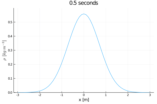
Diffusion 1D

Example examples/Diffusion_1D.jl will run a simple 1D diffustion equations:

$\\frac{\\partial \\rho}{\\partial t} = \\frac{\\partial^2 \\rho}{\\partial x^2}$ , where, $\\rho (x,t)$ is the density.

Using the embedded function shiftc which which returns a shifted value of the array, this example integrated for 12 seconds results:

Diffusion1D

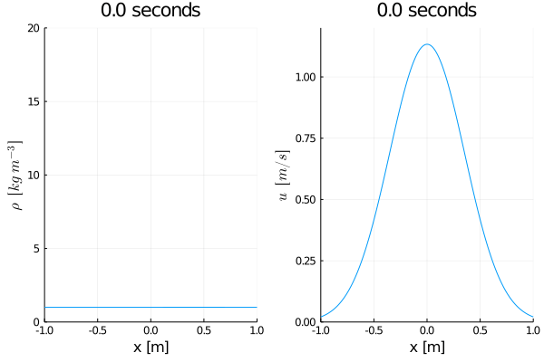
Advection 1D

Example examples/Advection_1D.jl will run a simple 1D Advection equations:

$\\frac{\\partial ( \\rho \\cdot \\u)}{\\partial t} = -u \\cdot \\frac{\\partial ( \\rho \\cdot \\u)}{\\partial x}$

$\\frac{\\partial \\rho}{\\partial t} = -\\frac{\\partial ( \\rho \\cdot u)}{\\partial x}$

where, $\\rho (x,t)$ and $u (x,t)$ are the density and x-dimension velocity fields.

Advection1D

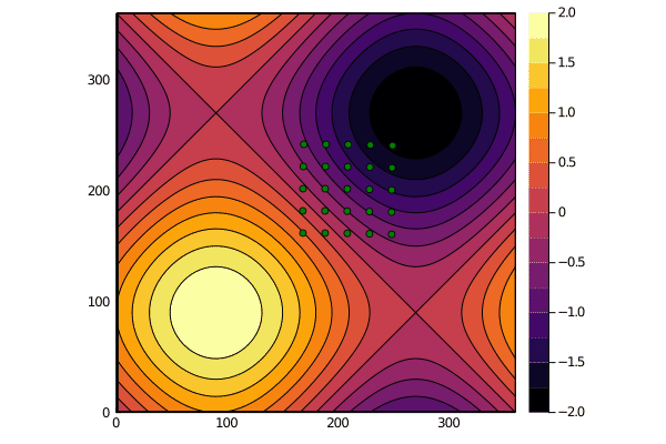
Random Flow

Example examples/RandomFlow_2D.jl simulates the trajectories of a particle cloud in a randomly generated flow field, given the stream function:

f(y,x) = sin(x) + sin(y)

Advection1D

Unbounded array

An additional CyclicArrays usage is for working with array that produce no BoundsError.

Define 1D grid with no connections:

nfaces=1;ndims=1;
faces=zeros(nfaces,ndims,2,4);
faces.=-1;

Define array:

x=[0:3;]
x1=CyclicArray(x,faces)

Then, for out of bounds indexes, CyclicArrays returns NaN:

julia> x1[0]
NaN